The default settings use basic OMP analysis with for water types representing ICW and AAMW based on potential temperature, salinity, oxygen, phosphate and nitrate. The summary at the end of the run should look like this:
P R O G R A M   R U N   S U M M A R Y :
---------------------------------------
Method used:   BASIC OMP ANALYSIS.
Dataset used:  testdata.
Upper limit of analysis:  0 dbar,
Lower limit of analysis:  6000 dbar.
Parameters used:
  potential temperature
  salinity
  oxygen
  phosphate
  nitrate
  mass conservation
Weights used (variables as listed):
    24
    24
     7
     2
     2
    24


Water types used:

 AAMW
 AAMW
  ICW
  ICW

Water type definitions for the selected variables and mass conservation

   10.0000   16.4000    9.0000   18.0000
   34.5600   34.5500   34.6500   35.8000
   91.0000  100.0000  260.0000  230.0000
    2.1000    1.4000    1.1000         0
   30.0000   19.0000   15.0000         0
    1.0000    1.0000    1.0000    1.0000

successfully analysed datapoints: 100 %

Print this summary for reference and check that the results make sense.
Press any key to see a graph of the mass conservation residual
against potential density.
You may want to verify at this stage how this selection corresponds to the settings found in incontr2.m and check that the run did select the correct water type definitions and weights from qwt2.m and testwght.mat.
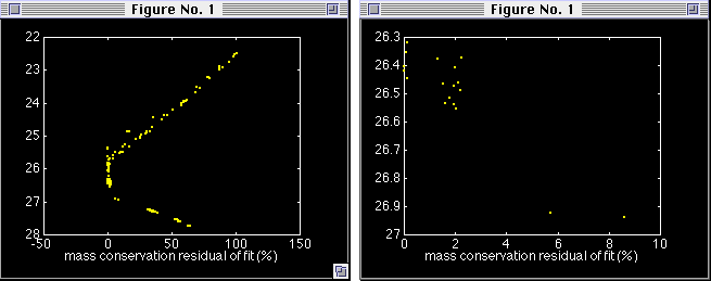
Pressing any key produces the figure at the left below. There is clearly a range where your analysis performs well, producing very small mass residuals; but over much of the range at the top and at the bottom the result is hopelessly bad. The reason is, of course, that you included only water masses of the permanent thermocline in the analysis but analysed data from the ocean surface to 6000 m depth. If you are only analysing for AAMW and ICW contributions you should restrict your analysis to the permanent thermocline.

Let us then run the analysis again, with the same data but restricting the depth range to 300 - 600 m (300 - 600 dbar). This is easily achieved in interactive mode; for automatic mode you have to edit incontr2.m before running the analysis again.
The result of the second run is shown in the right figure above. Note the different scales; most of your data points now give a mass residual of about 2%, and all results are well within 10%. A result such as this gives enough encouragement to check out the water mass fractions; they are shown below. The stations of this section were occupied from east to west, so east is on the left of the figures, which shows the largest contribution from the Indonesian Throughflow (AAMW).

It is always worth checking the quality of your water type definitions. To demonstrate the effect of changing the water type definitions we now run the analysis again, restricted as before to the 300 - 600 dbar range, with slightly different water type definitions for ICW. The default set qwt2.m contains a second set of ICW water type definitions for this purpose.
Run the analysis, using default settings except for the range, which you set to 300 - 600 dbar, and for the selected water types: When asked to give the water type numbers (rows in the water type matrix of qwt2.m) override the default 1, 2, 3 and 4 by responding with 1, 2, 5 and 6 (or [1 2 5 6] if you are using the graphical user interface). The figure below compares the results; the default is on the left, the result obtained with the new ICW definitions on the right. (The horizontal axis has been rescaled with the axis command from the command window to make the difference more visible.)
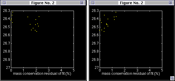
The new water type definitions reduce the magnitude of most residuals. This does not necessarily mean that the new definitions are a better representation of ICW; you have to remember that the ICW formation region is a long way from the region which we are analysing, and we are still using basic OMP analysis, ie we are not taking the effect of biogeochemical processes into account. All we are demonstrating is that proper definition of water types is a key aspect of OMP analysis.
If we are interested in reducing the large residuals which we obtained outside the 300 - 600 dbar range we have to include more water masses. Let us see how inclusion of AAIW improves the result.
Run the analysis again, using default values throughout except for the water type selection: When asked how many water types you want to include respond with 5. Enter 1, 2, 3, 4 and 7 for the water type numbers ([1 2 3 4 7] if you are using the graphical user interface). This will include AAIW along with the old ICW and AAMW in the analysis. The next figure compares the residuals from the default on the left (which includes only ICW and AAMW) with the new run on the right.
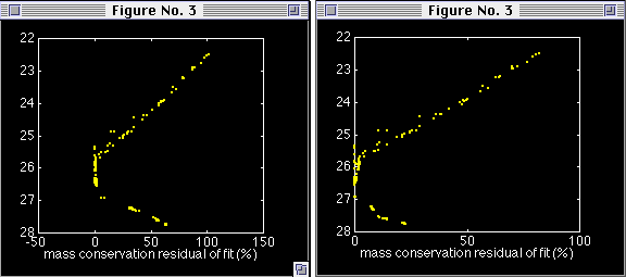
Nothing much changed at potential densities of 25.5 and less. This was to be expected, since inclusion of AAIW in the analysis can hardly help getting the upper 200 m of the water column right. The most prominent difference is the huge reduction in magnitude of the mass residuals below the 27 potential density level. This is clearly the result of including AAIW, which dominates the depth range below ICW and AAMW. But the magnitudes are still not acceptable in absolute terms. The reason for this is the same which is behind the slight deterioration of the result in the potential density range 25.5 - 27, biogeochemical processes acting on oxygen and the nutrients.
The most appropriate use of OMP analysis in the present situation (global scale analysis for water masses formed a long distance from the investigation region and use of water type definitions from the literature) is extended OMP analysis for ICW, AAMW and AAIW.
Run the program again, choose extended OMP analysis and follow the procedure of the last section in all other aspects. The result of this run is compared against the run from the last section in the next figure. The previous run (basic OMP analysis with five water types representing ICW, AAMW and AAIW) is on the left, the new run (extended OMP analysis) on the right. The horizontal axis has again been expanded to make the difference more visible. (The figure on the left is essentially a blow-up of the figure on the left above.)
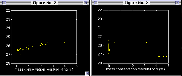
As we can see, we now have an excellent fit in the potential density range 25.5 - 27, which gives us confidence in the result. Below the 27 potential density level the fit is still not impressive, and we would have to look at our AAIW definition and possibly the inclusion of Circumpolar Deep Water there. However, this is only a demonstration of the method, and we do not pursue these aspects further but end the discussion by displaying the distributions of ICW, AAMW and AAIW along the section as derived in the last run:
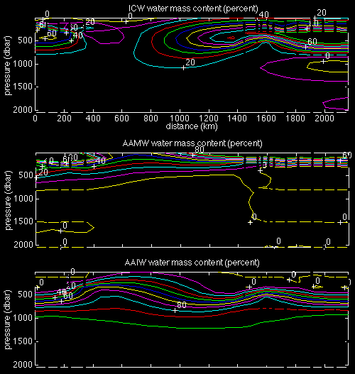
The result shows ICW dominating the permanent thermocline in the west, AAMW in the east and AAIW uniformly distributed along the section with its largest contribution below the 800 dbar level, falling off to zero at about the 500 dbar. Above 200 dbar the results are unreliable and show unrealistic distributions.
Reducing the mass residuals is of course also possible by simply changing the weight for mass conservation. The above examples were all derived with a mass conservation weight equal to the weight calculated for temperature (which usually has the largest weight). Conservation of mass is a concept and not a variable open to observation, so it is impossible to derive a mass conservation weight by calculation.
Which weight to allocate to mass conservation can be a matter of debate. Some argue that not conserving mass is physically unrealistic, and mass conservation should therefore have a significantly larger weight than all other parameters. How much larger this should be is then a matter of personal preference. It can also be argued that not conserving heat is as physically unrelistic as not conserving mass, so mass conservation should not be treated in a preferential manner.
The choice is essentially a personal one. We restrict ourselves here to pointing out that the subjective choice of the weight for mass conservation means that plots of mass residuals can therefore only be used as a relative indicator of the quality of a particular solution. The figure below demonstrates this by comparing the output from two runs with identical parameters but different mass conservation weights.
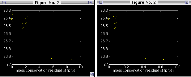
The left run is the default but restricted to 300 - 600 dbar, the right run is the same but with the mass conservation weight increased by a factor of 5. The weight used were [24 24 7 2 2 24] for the run on the left and [24 24 7 2 2 120] for the run on the right. Note the difference in scales.
There are many other aspects to OMP analysis which will only become apparent in practical applications. Generally, no OMP analysis should be performed without a detailed study of the distribution of residuals of individual parameters. A quick check is possible through the command plot(err(n,:),pdens), which produces the well known graphs of the mass residual against potential density for n = m (m = number of observed properties + 1). Other choices of n will produce equivalent graphs for potential temperature, salinity, oxygen etc. (The actual value of n for each property depends on the choice of observed properties for the program run.) A more detailed analysis would plot sections of property residuals in space. Regions with particularly large residuals in such a section plot can indicate problems with water type definitions.
Potential vorticity is a property related to the dynamics of the ocean. While it can be regarded to represent just another quasi-conservative tracer for which the weight is calculated in the same manner as for all other tracers, it also expresses the fact that movement in the deep ocean is quasi-geostrophic. This sets it apart from all other properties and could justify an independent setting of its weight. A more diffusive ocean would be modelled with a small weight for potential vorticity, while a more geostrophic ocean could be represented through a large weight. We and conclude this example by comparing the standard test run (which uses all default settings) with the same run when potential vorticity is included: Run the analysis again and click the potential vorticity button. The program will calculate potential vorticity from the testdata and include it in the analysis.
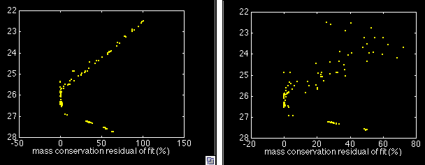
The figure on the left repeats the result from the standard test run, the figure on the right shows the result with the inclusion of potential vorticity. The example shows that potential vorticity can be used as a tracer, and the quality of the result is maintained even when potential vorticity receives the same weight as other conservative properties and mass conservation. Further investigation of residual distributions under different weighting schemes may reveal ocean regions which are more geostrophic than others. We invite users of OMP analysis to experiment in all directions.