OMP analysis is based on a simple model of linear mixing. It assumes that all water mass properties undergo the same mixing process, ie their mixing coefficients are identical (as this is the case in turbulent mixing). Their distribution in space can therefore be determined through a linear set of mixing equations.
The starting point of OMP analysis are observations of water mass parameters (such as temperature, salinity, oxygen etc). From these observations OMP analysis tries to determine the contributions from predefined source water types (SWT) which represent the parameter values of the "unmixed" source water masses. Mathematically OMP analysis is an inversion of an overdetermined system, performed individually for each observation point. All data points to be analyzed should therefore be located "downstream" from the source water masses, in other words on the spreading path of the water masses.
The SWT contributions or fractions xi for each data point are obtained by finding the best linear mixing combination in parameter space defined by temperature, salinity, oxygen, nutrients and other possible water mass properties which minimizes the residuals in a non-negative least squares sense (8). The solution includes two physically realistic constraints:
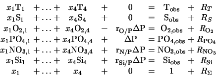
As an example we assume a mixing situation which involves four source water types and an observational data set which consists of the five parameters temperature, salinity, oxygen, phosphate and nitrate. The linear system of mixing equations which is the basis of classical OMP analysis (10; 18) is then given by

where the observed values of temperature Tobs , salinity Sobs , oxygen O2,obs , phosphate PO4,obs and nitrate NO3,obs with their respective residuals R define the columns on the right-hand side. The values Ti , Si , O2,i , PO4,obs and NO4,i (i = 1, ..., 4) represent the predetermined (known) parameter values of the four source water types for each parameter. The last row expresses the condition of mass conservation.
The above system of equations can be written in matrix notation as
Here, ![]() is the mean source water type of one parameter j calculated as:
is the mean source water type of one parameter j calculated as:

and sj is the standard deviation within each row, which is

The normalized variables are nondimensional, with zero mean and display a variation of order 1.
Normalization makes all parameters commensurable but does not necessarily make them all equally reliable for OMP analysis. Some parameters are difficult to measure and have a low instrumental or analytical accuracy; others may vary more in time and space than others and are therefore associated with high environmental variability. To account for these differences between parameters, all parameters are weighted.
Various procedures can be used to determine appropriate weights. Tomczak and Large (18) obtained weights by relating each parameter variance in the source water matrix G to a measure of the variance in the source region. They use the largest variance of the parameter in the source region dj max to obtain
Weighting procedures based on covariances between tracers due to variability of the source water types can be found in Mackas et al. (10). In our example we will use a mean variance in the source region obtained from the Matlab script polyval.m.
One way of accounting for biogeochemical processes is to convert non-conservative parameters into conservative parameters by introducing the "preformed" nutrients PO and NO (2; 20; 21). The same is achieved by adding another column to the water type matrix G which represents the biogeochemical transfer (6). The advantage of doing this is that the changes in the biogeochemical parameter field are obtained as an additional output from the analysis and that this information can be used to determine water mass age distributions. In both cases the rank of the matrix, compared with classical OMP analysis (section 2.1) is reduced by one; in the case of PO and NO because the oxygen information is used for the calculation of the two conservative parameters and therefore no longer available for the system of mixing equations, in the case of extended OMP analysis because the new unknown DP is added to resolve the biogeochemical changes:

The first two rows are the mixing equations for the two conservative parameters temperature and salinity which, not being affected by biogeochemistry, have zeros as their biogeochemical terms; the next four rows are the mixing equations for the nonconservative parameters oxygen and nutrients, and the last row expresses the condition of mass conservation.
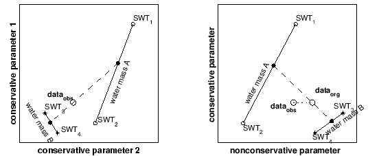
The new column on the left-hand side contains the Redfield ratios rO/P, rN/P and rSi/P, all referenced to phosphate, with DP the amount of biogeochemical change in phosphate (1; 13). Adding this column to the system of equations takes care of changes in source water type definitions due to biogeochemical influences (Figure 2.1).
 |
Figure 2.1 demonstrates the effect of introducing Redfield ratios with an example from the permanent thermocline where most water masses are described by a line defined through two water types. The mixing process between two water masses is then formally given by contributions from four source water types (SWT1, SWT2, SWT3 and SWT4). All points on the line between SWT1 and SWT2 form water mass A, all points on the line between SWT3 and SWT4 form water mass B. The four SWT contributions are found by a simultaneous solution in all parameter spaces (8). Figure 2.1 demonstrates how the extended OMP analysis proceeds in the case of two subspace combinations of conservative and nonconservative parameters. For two conservative parameters (left diagram), OMP analysis determines the contributions from all four SWTs directly. The contributions from SWT1 and SWT2 are added to represent the mixing fraction from water mass A; the contributions from SWT3 and SWT4 represent the contribution from water mass B. Mathematically the contributions from water mass A and B can be separated into contributions from their respective water types; graphically their contributions are found on the two lines between their respective SWTs and indicated as solid circles. The observational data dataobs represent the result of mixing between water masses A and B along the dashed line.
For a non-conservative parameter (right diagram) the observational data dataobs are also affected by biogeochemical processes. Introducing the Redfield ratio into the system of equations separates these effects from the conservative mixing solution, replacing the observational data dataobs by the corrected values dataorg.
We normalize the elements of Gext in the extended OMP analysis in two stages:

Here, the normalized ratio rpara/P' is obtained by relating the SWT values for j-th parameter of the classical OMP analysis (Gj) to the normalized classical SWT values (G'j) multiplied by the Redfield ratio rpara/P.
with N the Brunt - Väisälä frequency, f the Coriolis frequency and g the acceleration of gravity. In principle, this quantity can be evaluated from the temperature and salinity information supplied with the data, and the OMP analysis package includes the option to have potential vorticity calculated from the supplied data set. This is, however, not necessarily the most appropriate option. Data sets for OMP analysis are based on bottle data and therefore usually widely spaced along the vertical, which gives the calculation of the vertical density gradient (required for the calculation of N) from bottle data a somewhat low resolution.
Modern bottle data are usually collected from a CTD/rosette unit, and an alternative procedure could be to use the CTD temperature and salinity data for the calculation of potential vorticity and select the values found at the depth of the bottle data for inclusion in OMP analysis. This requires a separate calculation of potential vorticity from the CTD data before the OMP analysis package can be used. Potential vorticity then has to be supplied as one variable in the data set. (The OMP analysis package automatically checks for the presence of potential vorticity in the data set and only calculates potential vorticity from the bottle data if required. This is fully documented in the run summary at the end of the program run.)
As with all other parameters, the usefulness of potential vorticity depends crucially on the correct water type definitions, which cannot be found from the literature at present. Some investigative work is therefore required before potential vorticity can be included as another water mass tracer. This work may well go beyond the simple definition of source water type values. Here are a few aspects to consider, based on first experience.
Potential vorticity is a first-derivative quantity. (It includes the vertical density gradient.) This makes it a noisy quantity. Some filtering is usually necessary before it can be used as a tracer. Calculating potential vorticity from bottle data is equivalent to filtering. Potential vorticity derived from CTD data and filtered over a depth interval of 30 - 50 m does not differ all that much from potential vorticity derived from bottle data.
Potential vorticity as defined here changes its sign at the equator: When a water mass crosses the equator, the density structure remains more or less unchanged, which means that the Brunt - Väisälä frequency remains the same; but the Coriolis parameter changes its sign. This leads to a conundrum: How can a water mass change the sign of its potential vorticity? The answer is to be found in equatorial dynamics, which assigns an important role to relative vorticity and frictional effects. These aspects will be taken up in one of the next International WOCE Newsletters. In the meantime, please note that OMP Version 2 uses the absolute value of potential vorticity in all calculations.
Within the constraints of these remarks, first experience shows that the inclusion of potential vorticity in OMP analysis adds another tracer without degrading the result. This suggests that geostrophy and the OMP mixing model can be combined into a unified description of the oceanic water mass structure.